Peter Phaal and Sonia Panchen, sFlow.org
Packet-based sampling schemes are widely used to characterize network traffic. Packet sampling uses randomness in the sampling process to prevents synchronization with any periodic patterns in the traffic. On average, 1 in every N packets is captured and analyzed.
While this type of packet sampling does not provide a 100% accurate result, it does provide a result with quantifiable accuracy. This paper provides examples and describes the basic techniques used to calculate results and quantify accuracy when processing packet sample data.
Suppose 1,000,000 packets transit the network. A random sample of 0.25% is taken (2,500 packets). If 1,000 of the samples represent a particular class of traffic, voice traffic say, then how many of the 1,000,000 packets were actually voice packets? At least 1000 must have been voice packets because they have been seen in samples. The greatest number of voice packets that could have been sent is 998,500 because 1,500 samples have been seen that were not voice packets. However, neither of these two values is at all likely. It is most likely that the fraction of voice traffic is in the same ratio as its fraction of the samples i.e. 40% (1,000 divided by 2,500). This gives a value of 400,000 frames as the best estimate of the total number of voice packets.
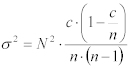
Generally, if there are a total number of packets, N, and a total number of samples, n, of which a certain number belong to a particular class, c, then the number of frames in the class,Of course it is very unlikely that there were exactly 400,000 voice packets. Instead a small range of values can be specified that are very likely, say 95% likely, to contain the actual value. In this case one can be 95% confidant that the actual number of voice was between 381,000 and 419,000.
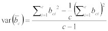
The following equation allows the variance of the estimate ofThe 95% confidence interval for ![]() is thus:
is thus:
Another way of expressing this range is as a percentage of the most likely value, so one might say that 400,000 packets +/- 4.8% voice frames were sent, or in other words that the largest likely error is 4.8%.
The following equation provides a simple estimate of the percentage error:Plotting this equation as a chart shows how sampling accuracy improves as c increases.
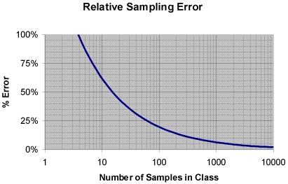
Chart 1: Relative Sampling Error
One can read off the percentage error for the example where c was 1,000. This gives approximately 6%.
An interesting thing to notice is that the accuracy of measurements doesn't depend on the total number of frames, but simply on the number of samples used to make the measurement. This property is very useful when monitoring high-speed switches or routers. For example, suppose one is monitoring a small switch, with traffic averaging at 400 frames/second, using a sampling rate of 0.25%. One can get the same level of accuracy monitoring a fast switch with a frame rate of 40,000 frames/second using a sampling rate of only 0.0025%.
Statistical sampling can produce results that vary significantly around the true value when measurement intervals are short, or when the traffic rates are very low. This effect is best illustrated by an example.
Suppose that voice traffic is being transmitted at a rate of one packet per second and that is has been monitored for an hour. There will end up being 3,600 voice packets in the hour. If the sampling rate was set to 0.25% then one should see approximately 9 samples of voice packets. The percentage error in this case works out to be 65%. This means that one can expect to see hourly estimates of the number of voice packets ranging between 1,200 and 6,000 packets.
There are two ways that the accuracy can be improved. The first way is to increase the sampling rate. Suppose the sampling rate is increased to 1%. One should then see approximately 36 samples of voice packets in an hour and get a percentage error of about 33% and so one would expect to see hourly estimates in the narrower range of between 2,400 and 4,800 packets. Care needs to be taken when increasing the sampling rate as it also increases the amount of sample traffic on the network and the amount of work that needs to be performed to analyze the samples.
The other way to see improved accuracy is to look at the data over a longer period of time. If a monthly analysis is run using the original 0.25% sampling rate one would expect to see around 6,700 samples of voice packets in the month. This gives a percentage error of only 2.4% with monthly estimates in the range 2,610,000 to 2,740,000 packets. Thus, one may want to use longer periods, such as weeks or months, to do things like billing for network usage, which require more accurate data.
In most cases sampling works out well. Large sources of traffic are estimated with sufficient accuracy in short intervals to make real-time congestion management effective. Applications, such as usage billing and capacity planning, that require greater accuracy make use of data collected over longer periods and so achieve reasonable accuracy.Packet sampling can be modeled by the Binomial Distribution. There is a good explanation of the binomial distribution at on the Yale University Department of Statistics web site.
The binomial distribution describes the behavior of a count variable, c, if:
If these conditions are met, then c has a binomial distribution with parameters n and p. The following equations calculate the mean and variance for the binomial distribution:
For packet sampling we do not know the population proportion (i.e. probability, p, that a sample belongs to a class), but we observe the sample proportion i.e. the count of "successes" divided by the number of observations:
where:
| P = sample proportion | |
| c = number of samples in a given class ("successes") | |
| n = number of samples |
Jedwab et. al. demonstrated that condition 4. is satisfied for any random packet sampling function. Thus, if we know that the count, c, of "successes" in a group of n observations with success probability p, has a binomial distribution, then we are able to derive information about the distribution of the sample proportion, P.
By the multiplicative properties of the mean, the mean of the distribution of P is the mean of the distribution of c divided by n:
Thus the sample proportion, P, is an unbiased estimator of the population proportion, p.
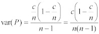
The variance of P is equal to the variance of c divided by n. The variance of a random variable multiplied by a constant is given by the equation:
thus:
If the number of samples, n, is large, then sample proportion is approximately a Normal Distribution with mean of p and variance of p(1-p)/n, by the Central Limit Theorem.
Using these approximations, the maximum likelihood estimate of p (the population proportion) is the sample proportion, P. And the variance of the sample population is an unbiased estimate of the variance of the population proportion:
Note: The divisor is (n-1) rather than n because we are now dealing with a measured statistic, rather than a probability from a known distribution. A news group posting by David Seal to sci.math provides a more detailed explanation.
However, we are interested in the variance in the estimate of the total number
of frames in the class, ![]() , where:
, where:
where:
| N is the total number of frames. |
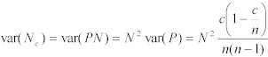
The variance of the estimate of ![]() is thus:
is thus:
The 95% confidence interval for ![]() is thus:
is thus:
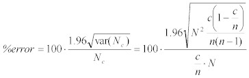
Another way of expressing this range is as a percentage of the most likely value.
which simplifies to:
Typically n >> c. This gives the equation:
The previous equations all dealt with estimating packet counts. Often it is useful to estimate the bytes consumed by a particular class. Byte estimates are easily computed using the following equation:
where:
The average packet size and the variance in the packet size are easily calculated using the equations:
and
When multiplying two random variables, the variance of the product can be obtained using the following equation:
Applying the equation to ![]() gives the result:
gives the result: